ctsem fits continuous and discrete time state space models to longitudinal data. A system of stochastic differential equations (or difference equations, in discrete time) describes how a set of latent processes change and affect each other, and a measurement model links those processes to the observed variables. Panel data with a few waves, intensive longitudinal data with hundreds of observations per person, and single long time series all use the same interface, and observation times can be irregular and different for every person.
Version 4 fits with a new engine written in Julia by default. For what changed since 3.x, see New in 4.x.
What it covers
- Dynamics. Several interacting processes, higher order dynamics such as damped oscillation, time dependent inputs and interventions, and parameters that depend on the latent state (nonlinear dynamics). Latent growth curves, latent change scores and the cross-lagged panel model are special cases.
- Measurement. Several indicators per process, as in dynamic factor analysis. Indicators can be continuous, binary, ordinal, counts or censored, mixed within one model, and loadings, intercepts and error variances can depend on the latent state.
- Individual differences. Any parameter can vary between people, or at several nested levels such as people within couples, and depend on time independent covariates, linearly or as a smooth function. Random effects are integrated out by a Laplace approximation, exactly wherever they shift a mean in a linear Gaussian model, and each fit checks the approximation’s error for every person and warns where it would change the estimates.
- Estimation and uncertainty. Maximum likelihood, or maximum a posteriori with priors, using exact gradients; standard errors from the Hessian along with a check of the normal approximation; or sampling of the full posterior, random effects included.
- Speed. On one core, the first example below fits in 18 seconds with the Julia engine and 56 with Stan, and a simulated panel of 400 people with 40 observations each in 18 against 47, each pair reaching the same maximum (timings: one AMD EPYC 9654 server, November 2026).
-
Threads. The likelihood, its gradient and the Hessian are computed in parallel over subjects within one process, so
coresspeeds up a single fit. With random auto-effects added to that panel, a fit took 637 seconds on one core, 173 on four and 60 on sixteen. - No compiling per model. The engine is compiled once, the first time it is used after installing. A nonlinear version of the first example then fitted in 64 seconds in a new R session, while Stan spent about six minutes compiling the same model, in every new session, before a 76 second fit.
-
Checking and building models. Score tests for what a model leaves out, tests of its one-step-ahead prediction errors, cross validation, identification checks before fitting, and a step-by-step model search.
ctReport()runs the reporting and checking functions over a fit and writes the results to a folder.
Install
install.packages('ctsem')    # the released version, from CRAN

# or the development version, which is what this page describes
remotes::install_github('cdriveraus/ctsem',
  INSTALL_opts = "--no-multiarch", dependencies = c("Depends", "Imports"))
Then, once:
ctJuliaInstall() installs whatever is missing: Julia itself, the JuliaConnectoR package that links it to R, and the engine’s Julia packages. It asks before each download. The first fit after installing or updating ctsem builds a compiled image of the engine, which takes several minutes; after that each R session starts the engine in a few seconds. ctJuliaStatus() reports what was found.
Without Julia, ctFit(..., backend = 'stan') fits with Stan as ctsem 3.x did, but most of what is new in version 4 needs the Julia engine.
Compile problems on Windows (rstan / Rtools)
Installing from GitHub compiles ctsem’s Stan models, and with backend = 'stan' a nonlinear model is compiled before it is fitted. Both need a working C++ toolchain. Ensure a recent R and a matching Rtools are installed, and check that rstan itself works before suspecting ctsem.
Put this single line in ~/.R/Makevars.win, deleting any other lines:
If you see errors like g++ not found, install devtools, which brings the toolchain checks with it:
install.packages('devtools')For anything else compiler related, the Stan forums are the best place to look: https://discourse.mc-stan.org/.
A first model
Two coupled processes, densely measured. milkman_rdm1 in the doBy package records daily milk yield and fat percentage through a full lactation for 53 dairy cows, a median of 230 observations each. That density is what makes individual differences in the dynamics estimable at all, rather than only differences in level.
library(ctsem)
data(milkman_rdm1, package = 'doBy')

milk <- data.frame(
  cow   = milkman_rdm1$cowno,
  day   = milkman_rdm1$dfc,                     # days since calving
  yield = as.numeric(scale(milkman_rdm1$my)),
  fat   = as.numeric(scale(milkman_rdm1$fatpct)))

model <- ctModel(
  type = 'ct',                        # 'dt' for the discrete time equivalent
  LAMBDA = diag(2),                   # two processes, one indicator each
  manifestNames = c('yield', 'fat'),
  latentNames = c('yield', 'fat'),
  time = 'day',
  id = 'cow')

fit <- ctFit(milk, model)
Nothing there is constrained. LAMBDA is the factor loading matrix linking latent processes to observed variables, and its dimensions are what tell ctsem the system has two processes with one indicator each. Every other matrix – the auto and cross effects, the system noise and its correlation, the measurement error, the initial states – takes a default and is freely estimated, with individual differences where ctsem’s defaults put them. Scaling the two variables, as above, makes for easier estimation and more sensible default priors.
summary(fit)$popmeans
#>                   mean    sd   2.5%    50%  97.5%   mode
#> T0m_yield       -0.942 0.146 -1.232 -0.944 -0.646 -0.943
#> T0m_fat          0.145 0.198 -0.241  0.139  0.527  0.150
#> drift_yield     -0.041 0.004 -0.050 -0.040 -0.033 -0.041
#> drift_yield_fat -0.020 0.004 -0.028 -0.020 -0.012 -0.020
#> drift_fat_yield -0.006 0.003 -0.012 -0.006  0.001 -0.006
#> drift_fat       -0.015 0.004 -0.025 -0.015 -0.009 -0.015
#> diff_yield       0.136 0.004  0.129  0.136  0.143  0.136
#> diff_fat_yield  -0.595 0.058 -0.703 -0.595 -0.480 -0.592
#> diff_fat         0.116 0.005  0.106  0.115  0.125  0.116
#> mvaryield        0.329 0.003  0.323  0.328  0.335  0.328
#> mvarfat          0.582 0.005  0.574  0.582  0.591  0.582
#> mm_yield        -0.059 0.124 -0.303 -0.062  0.178 -0.054
#> mm_fat           0.148 0.112 -0.075  0.142  0.357  0.142
Drift names read as drift_<affected>_<predictor>, so drift_yield is yield’s own auto effect and drift_yield_fat is the effect of fat on yield. A negative auto effect pulls a process back toward its equilibrium and its size sets how fast. diff_yield and diff_fat are the system noise standard deviations, and diff_fat_yield is the parameter behind their correlation; the correlation itself, -0.53, is the DIFFUSIONcor row of summary(fit)$parmatrices. mvar* are the measurement error standard deviations, and T0m_* the mean initial states.
The two cross effects are not symmetric: a high fat percentage predicts a subsequent fall in yield, and the interval for drift_yield_fat excludes zero, while the interval for the reverse effect does not.
summary(fit)$popsd
#>            mean    sd  2.5%   50% 97.5%  mode
#> T0m_yield 0.899 0.119 0.688 0.896 1.146 0.892
#> T0m_fat   1.155 0.155 0.863 1.153 1.455 1.149
#> mm_yield  0.750 0.107 0.559 0.742 0.980 0.742
#> mm_fat    0.425 0.257 0.117 0.370 1.102 0.366
Those are the population standard deviations of the parameters that vary by cow. ctsem’s defaults put random effects on the initial state and the observation intercept; adding indvarying to a parameter’s specification puts them elsewhere, on an auto effect or a cross effect, which is what the density of this data buys.
To read the model as equations rather than as code, ctModelLatex(model) renders it to pdf or png.
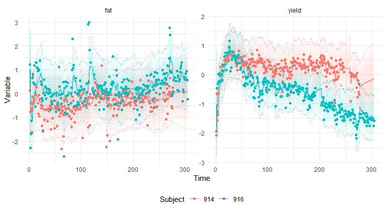
Points are the observations, lines the model’s expectation for each cow, and the bands its uncertainty. The rise and slow decline in yield is the lactation curve, which the model is picking up as a long deviation from equilibrium rather than as a trend term.
ctDiscretePars(fit, plot = TRUE)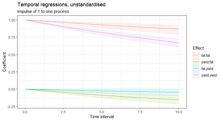
This last plot is the thing continuous time gives you. The same estimated system is expressed as regression coefficients at every interval between observations, instead of only at the one interval a discrete time model happens to be fitted at. Over the ten days shown, the effect of fat on yield keeps accumulating while the reverse effect stays flat and near zero.
Covariate effects on parameters
Something closer to real use: chick growth under four diets, asking whether diet moves a parameter of the process rather than only the observed mean. ChickWeight is in base R.
chickdata <- ChickWeight
# Diet is categorical, so it needs dummy / 'one hot' coding.
chickdata <- cbind(chickdata, model.matrix(~ Diet - 1, chickdata))
colnames(chickdata)[5:8] <- paste0('Diet_', 1:4)
# Scaling continuous variables makes for easier estimation and more sensible
# default priors. Time intervals can benefit too.
chickdata$weight <- scale(chickdata$weight)
head(chickdata, 3)
#>       weight Time Chick Diet Diet_1 Diet_2 Diet_3 Diet_4
#> 1 -1.1230637    0     1    1      1      0      0      0
#> 2 -0.9964315    2     1    1      1      0      0      0
#> 3 -0.8838695    4     1    1      1      0      0      0
m <- ctModel(
  type = 'ct',
  LAMBDA = diag(1),
  manifestNames = 'weight',
  latentNames = 'Lweight',
  time = 'Time',
  id = 'Chick',
  DRIFT = 'a11, transform=param',              # lift the usual sign restriction
  MANIFESTMEANS = 0,                           # identification: fix one of
  CINT = 'cint, tipreds=c(Diet_2,Diet_3,Diet_4)',   # these two, estimate the other
  TIpredNames = paste0('Diet_', 2:4),          # diet 1 is the baseline
  tipredDefault = FALSE)                       # only the effects asked for

f <- ctFit(chickdata, m, priors = TRUE)
Priors are used here because the model is only weakly identified by these data without them: growth over a dozen observations does not pin down an auto effect and a continuous intercept independently.
Two pieces of syntax recur everywhere and are worth unpacking:
A string is a free parameter, a number is a fixed value. The observation intercept and the process intercept cannot both be free – they describe the same level – so
MANIFESTMEANS = 0is what letsCINTbe estimated.-
A parameter carries options after its name, as named fields. The fields are
transform,indvarying(random effects),sdscale(the random effect sd prior relative to the mean’s) andtipreds(covariate effects); anything not named takes its default. So'cint, tipreds=c(Diet_2,Diet_3,Diet_4)'is a parameter namedcint, default in every other respect, moderated by three columns.The same cell can be written positionally, with
|separating the fields in that order:'cint ||||Diet_2,Diet_3,Diet_4'builds an identical model. That is the form the manual and older code use, andctPar()writes it for you from named arguments.
summary(f)$tipreds
#>                  mean    sd   2.5%   50% 97.5%  mode     z
#> tip_Diet_2_cint 0.021 0.013 -0.004 0.020 0.046 0.021 1.608
#> tip_Diet_3_cint 0.050 0.013  0.025 0.050 0.077 0.051 3.840
#> tip_Diet_4_cint 0.028 0.013  0.002 0.028 0.052 0.028 2.128
Diets 3 and 4 raise the continuous intercept clearly; diet 2 is not distinguishable from the baseline diet.
# One chick per diet, predicted from the covariates alone rather than from data.
ctPredict(f, plot = TRUE, removeObs = TRUE, polygonalpha = 0,
  subjects = as.numeric(chickdata$Chick[!duplicated(ChickWeight$Diet)]))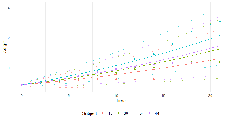
# Temporal regression coefficients as a function of the time interval.
ctDiscretePars(f, plot = TRUE)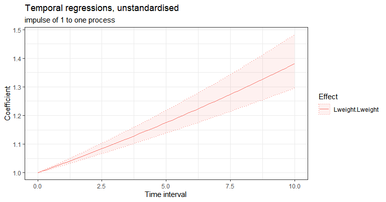
Because the sign restriction on the auto effect was lifted, the coefficient rises above one as the interval grows: an increase in weight promotes further increase, which is what growth looks like in this parameterisation.
Where to go next
| If you want to | Read |
|---|---|
| Read the help pages, vignettes and changes in a browser | the ctsem website |
| Know what changed since ctsem 3.x | New in 4.x |
| Understand what a dynamic system is, and why it is worth the trouble | Dynamic systems modeling in psychology |
| Work an applied example end to end, from theory through simulation to fitting and checking | the tutorial preprint, with code and materials in the OSF project |
| A second, shorter worked start | ctsem quick start: sunspots and a damped linear oscillator |
| Get everything ctsem can say about a fit, in one folder | ctReport(fit) |
| The full reference: the model, the priors, every argument | the hierarchical manual (pdf), or ctDocs() in R |
| Understand and control the uncertainty ctsem reports | uncertainty vignette |
| Build a measurement model: multiple indicators, binary, ordinal, count or censored items | measurement models vignette |
| Put random effects on parameters, at one or several levels | multilevel Laplace vignette |
| Model test items as indicators: item response models over time | IRT items vignette |
| Decide whether to treat a rating scale as ordinal or continuous | ordinal or continuous vignette |
| Find out what a fitted model is missing | score tests vignette |
| Weight subjects to represent a population | sampling weights vignette |
| Fit each subject separately, with the population estimate as a prior | empirical Bayes vignette |
| Fit discrete time models, and know when the choice matters | Discrete time models using ctsem? and Representations of dynamic systems |
| Handle an accelerated longitudinal or multiple group design | Accelerated longitudinal and multiple group designs |
| Understand missingness, and filtered against smoothed estimates | Kalman filter vs smoother |
| Think about individual differences and what heterogeneity means | What is heterogeneity, really? and the conceptual paper |
| Model an intervention or another external input | Understanding the time course of interventions |
| Fit a growth curve with state dependent error | Latent growth curves, state dependent error |
| Work with binary observations | Binary data in state space models |
| Point and click instead of writing code | ctsemGUI, a Shiny front end |
| Use the original OpenMx based ctsem (version 1 style) | ctsemOMX and its vignette |
Function map
The functions most users need, by task. ?name gives the details for any of them.
Specify a model
ctModel |
specify a continuous (type = 'ct') or discrete ('dt') time model |
ctModelLatex |
render the model as equations, to pdf or png |
model$matrices |
view and edit the specification in matrix form, e.g. model$matrices$DRIFT[1, 2] <- 'cross'
|
ctPar |
write a cell specification from named arguments |
ctCov |
write a covariance matrix as the cells a model reads |
ctModelHigherOrder |
raise the order of a model, for instance to allow oscillation |
ctModelSlowComponent, ctModelPeriodicComponent, ctModelUniqueProcess, ctModelLatentLevel
|
add a slow process, a cycle, an indicator specific process, or carry levels in the latent processes |
ctModelConvertOMX |
convert an old OpenMx style (type = 'omx') model object |
ctIdentify |
check which parameters a dataset can inform, before fitting |
Prepare data
ctWideToLong, ctLongToWide
|
reshape between wide and long format |
ctIntervalise, ctDeintervalise
|
convert between absolute times and intervals |
ctDiscretiseData |
bin long format observations onto a chosen grid |
Fit
ctFit |
fit a model: maximum likelihood, maximum a posteriori, or sampling |
ctFitUpdate |
refit with changed data or arguments |
ctFitUncertainty |
recompute a fit’s uncertainty (Hessian, checked, importance sampling, sandwich, bootstrap), refine its random effects by quadrature, or sample its posterior with ctFitUncertainty(fit, 'sample')
|
ctEmpiricalBayesFit |
subject-wise fits with the population estimate as a prior |
Inspect a fit
summary, coef, vcov, logLik
|
estimates, random effect sds, covariate effects, residual covariance |
ctSummaryMatrices |
the dynamic system parameters in matrix form |
ctSubjectPars |
subject specific parameters |
ctExtract |
the raw draws, as named arrays |
ctPlotPosterior |
prior against posterior, per parameter |
ctTIpredEffects, ctPredictTIP
|
covariate effects on parameters, and on expected observations |
ctDiscretePars, ctDiscreteParsPlot
|
temporal regressions as a function of the time interval |
ctNetwork, ctNetworkPlot
|
temporal and contemporaneous networks of the fitted system |
ctPhasePortrait |
phase portrait of the fitted dynamics |
ctStateDependencePlot |
how model matrix cells vary with a latent state, for nonlinear models |
ctVarianceDecomposition |
split each indicator’s variance into between person, process and measurement parts |
ctTracePlot |
the optimisation path, or the sampling chains, of a fit |
Predict
ctPredict |
predictions and uncertainty, conditional on all, some, or none of the data |
ctKalman, ctKalmanArray
|
filtered and smoothed state estimates |
ctResiduals |
standardised residuals |
Check, compare and improve
ctReport |
run the reporting and fit-checking functions over a fit and write a folder, with an index saying how to read each file |
ctScoreTest |
test, without refitting, whether random effects, covariate effects or state dependence are missing |
ctFitAdequacy |
tests of the one-step-ahead prediction errors, grouped by what they detect |
ctModelImprove, ctModelProposals
|
step-by-step model search guided by those tests |
ctPostPredPlots |
posterior predictive comparison of implied and observed data |
ctFitCheckCov |
lagged covariance diagnostics |
ctACF, ctACFresiduals
|
continuous time autocorrelation, of the data and of the residuals |
anova, ctChisqTest
|
compare nested fits |
ctLOO |
cross validation: k fold by refitting, or PSIS for Laplace fits |
ctFitProfile |
profile likelihood of chosen parameters, for identification and intervals |
ctLaplaceCheck |
measure the Laplace approximation error for random effects; ctFitUncertainty(fit, intoverpop = 'quadrature') corrects it |
ctParticleLik |
measure the filter’s approximation error against a particle filter; ctFitUncertainty(fit, 'is', filter = 'particle') corrects the draws for it |
ctCoverageCheck |
generate from a model, refit repeatedly, and check parameter recovery |
Generate data
ctGenerate |
from a model, at given parameter values or (fromPriors = TRUE) drawing them from the priors |
ctGenerateFromFit |
from a fitted model |
Julia engine
ctJuliaInstall |
install Julia, the bridge package, and the engine’s dependencies |
ctJuliaStatus |
report whether the Julia engine is available |
ctJuliaSetup |
configure the Julia session: its thread count, or a particular Julia installation |
ctJuliaProcesses, ctJuliaKill
|
list, and stop, the Julia processes ctsem has started |
Getting help
Questions, and the answers to a good many earlier ones, are at https://github.com/cdriveraus/ctsem/discussions. Bug reports belong in issues.
To cite ctsem, run citation('ctsem').
Older function names
From version 3.11.0 the user facing functions dropped their Stan specific wording. Existing code keeps working: the old names remain as aliases.
ctFit() is the main fitting function and ctStanFit() is an alias of it. Its second argument is now model; the older ctstanmodel is deprecated but still accepted. ctModelConvertOMX() replaces ctStanModel() for converting old OpenMx style model objects. Otherwise:
Project history
Version 1 of ctsem provided SEM based functionality by linking to OpenMx, which allowed random means but fixed regression and variance parameters across subjects. Those functions now live in the separate ctsemOMX package, documented in a JSS publication (Driver, Voelkle & Oud, 2017) and its vignette.
Version 2 introduced the hierarchical specification and a Kalman filter coded in Stan, letting every parameter of the dynamic model vary across individuals with an estimated population mean and variance. Version 3 added state dependent (time varying) parameters. Version 4 added the Julia engine, and with it Laplace integration of random effects, nested levels, and ordinal, count and censored indicators. For most purposes the current formulation is faster, more robust and more flexible than the OpenMx one; with many subjects, few time points and no individual differences in timing, ctsemOMX can still be quicker.
Changes, version by version, are in NEWS.md; New in 4.x describes version 4 for users of 3.x.